Archive · Simulation note · XR1-SIM-004 · REV B
The wake solver
The model's first job is not to fly the aircraft. It is to predict the wake of one sector on a thrust stand.
REV A described a lattice-Boltzmann magnetohydrodynamics code running inside the vehicle, faster than the plasma evolves, as the heart of a flight controller. The method was sound; the job was wrong. A vehicle cannot be controlled by a model nobody has checked, and nothing has been checked until a sector has produced a wake and someone has measured it. REV B moves the solver to where it earns its keep: the test hall, one gate ahead of the hardware.
The method
The lattice-Boltzmann method evolves particle distribution functions $f_i(\mathbf x,t)$ along a small set of discrete velocities $\mathbf c_i$ on a regular lattice. Each step streams populations to neighbouring nodes and relaxes them toward a local equilibrium:
The relaxation is the Bhatnagar–Gross–Krook collision operator (1954); the three-dimensional nineteen-velocity lattice, D3Q19, is from Qian, d'Humières and Lallemand (1992). A Chapman–Enskog expansion shows that density and momentum moments recover the weakly compressible Navier–Stokes equations when the Mach number is small. Every node updates from its neighbours alone: no global pressure solve, no matrix inversion, and a structure that maps directly onto graphics processors. Established physics
The electromagnetic body force enters through the forcing term $F_i$. The discrete form matters; Guo, Zheng and Shi (2002) showed which forcing scheme recovers the intended momentum equation without spurious lattice artifacts.
Why it fits this problem
Low Mach number. The hover benchmark puts the induced velocity at 22.6 m/s and the far wake at 45.2 m/s: Mach 0.07 to 0.13. Compressibility error in the standard scheme scales with the square of the Mach number, about 2% at the top of that range.
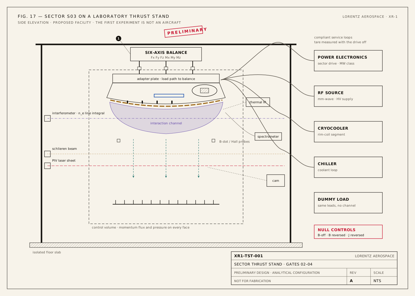
Awkward geometry. A sector on a thrust stand sits in a hall with a floor, walls, a balance frame, cable runs and a diagnostic gantry, all of which shape the wake that the PIV sheet will see. Bounce-back boundaries put that geometry on the lattice without body-fitted meshing.
A known force field. At $R_m\sim10^{-5}$ the magnetic field is the coils' vacuum field (XR1-SIM-002), computed once. REV A carried a second distribution to evolve $\mathbf B$ through the induction equation, following Dellar (2002). That machinery is correct for conducting fluids at larger $R_m$, and unnecessary here: the flow solver needs only the force density $\mathbf J\times\mathbf B$ on its lattice. Established physics
What it cannot do alone
The force density comes from somewhere else. A separate electrical and plasma-chemistry solver must supply the current: charge conservation with an anisotropic conductivity, electron production by the millimetre-wave source, and loss by attachment and recombination (XR1-TR-003). The coupling runs both ways but weakly at hover speeds, where the motional field $\mathbf u\times\mathbf B$ is about 0.2 kV/m at 45 m/s in 5 T.
Heat is part of the answer. At the conductivity and volume in XR1-CALC-002, Joule dissipation averages about 150 kW per cubic metre of interaction region. Heated air is lighter; it rises, and a rising plume on a balance looks like thrust. The solver therefore carries an energy equation and buoyancy, for the same reason Gate 02 carries thermal controls. Simulation target
Turbulence is not resolved. The wake Reynolds number, $Re=UL/\nu$, is about $3\times10^{6}$ at 45 m/s over a metre. The solver runs as a large-eddy simulation with a subgrid model; it predicts mean wake velocity and momentum flux, not every eddy.
A sizing check. A 10 × 10 × 20 m domain around one sector at 2 cm spacing is 250 million nodes; nineteen single-precision populations per node is about 19 GB of population state. That is a workstation-class GPU cluster problem, not a supercomputer one. A domain estimate, not a converged mesh.
Validation before prediction
| Step | Solver input | Compared against |
|---|---|---|
| V1 | No force; a jet or wake of known geometry | Published benchmark flows |
| V2 | Heat source only, magnet off | Gate 02 thermal controls: the plume and the balance reading with B off |
| V3 | Body force from the measured current distribution | Gate 03 wake: PIV and schlieren, momentum flux, temperature |
| V4 | Two or more sectors, differential power | Gate 05 control tests |
Only after V3 agrees with measurement does the solver's prediction for a full annulus mean anything, and even then it is a prediction with stated uncertainty, not a result. Reduced-order surrogates for control (XR1-SIM-003) are trained against the validated solver and the measured discharges, never against the solver alone. Simulation target
Revision notes
| REV A (2025) | REV B |
|---|---|
| Onboard digital twin inside the flight controller | Ground solver for the test program; flight software is out of scope until Gate 05 |
| Full MHD lattice-Boltzmann with a magnetic distribution function | Flow solver with an imposed-field body force; induction is negligible at $R_m\sim10^{-5}$ |
| Update rates and processor specifications for a flight unit | Withdrawn; no such hardware exists |
| Calibration against in-flight plasma diagnostics | Validation against Gate 01 to 03 measurements on the stand |
A simulation is a hypothesis with good bookkeeping. The thrust stand decides whether it is right.